2. Deformable Surface Algorithm
2.1 The Algorithm
The idea of this algorithm is borrowed from the surface model. For a warping from X to X', (X' - X) is viewed as a function of X: X' - X = (dx(x, y), dy(x, y)).
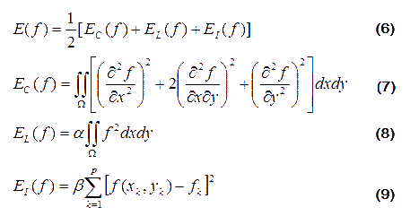
Consider a function f on the 2D plane (x, y) (e.g. f = dx or f = dy in this algorithm), and the enengy minimization objective functional is
where (7) requires the curvature of this surface is small, (8) is a regularization term and (9) utilizes the function values at some points which are known (in this algorithm these points are control points).
The optimal function f can be obtained from the Eular-Lagrange equation
(11)
We add Neumann boundary condition to this equation in the original paper:
The discrete form of this equation is
Af = b (12)
The discretization of the partial derivatives part is a 5x5 filter
Then we can obtain dx, dy, i.e. the warping, independently by solving (12).
2.2 Implementation
A. Interpolation after Mapping Computation v.s. Mapping Computation after Interpolation
My implementation is different from the original paper [2].
In [2], it is suggested to compute the mapping from the left image to the right image W0 and the mapping from the right image to the left image W1. Then use forward mapping
W0 (t) = t W0,
W1 (t) = (1-t) W1
to warp the left image and the right image to the morphed image at the time t, respectively. However, the forward mapping has problems as discussed in Section 1.1-D.
So I suggest two ways of implementation (the second one is the final choice in the implementation):
(1) Compute W0 and W1. Then use reverse mapping
W0 (t) = t W1,
W1 (t) = (1-t) W0
to warp the left image and the right image to the morphed image at the time t, respectively.
The advantages of this approach are:
First, we only need to solve the four groups of linear equations once, when rendering a movie;
Second, the warping is consistent along the time axis t.
While the disadvantages are:
First, the warping is not good when there are a significant rotations between two images, as the interpolation of mappings is linear (Fig. 8).
Warp using (1)
Left Image Right Image
Warp using (2)
Fig. 8 The comparison of two warping computation methods when there is a rotation between two images.
Second, we only utilize the control points but not utilize the line segments.
(2) Using the interpolation methods of the control line segments to get a control line segment in the morphed image. Then compute the reverse mapping W0(t) and W1(t) independently, with the corresponding line segments in the morphed image and the source images.
The advantages of this approach are:
First, the computational cost is lower when using the acceleration technique via LU factorization introduced in Section 2.2-B.
Second, we utilize the line segments, to make the computation more robust.
While the disadvantage is:
First, the computational cost is much higher when rendering a movie.
Second, the warping is NOT consistent along the time axis t (Fig. 9). This may be solved by utilizing the optimal flow techniques.
Warp using (1) Warp using (2)
Fig. 9 The comparison of two warping computation methods on the time consistency.
B. The Acceleration Issues
The major computational cost is the step of solving linear systems. We accelerate this step from two aspects.
1) Use LU factorization to solve the linear system. First, decompose A as A = LU. Then solve Ly = b and Ux = y. The first step needs much more time than the second one.
As the left side A is the same for all the four groups of linear equations, if the time t, i.e. the line segments in the morphed image is determined, only one LU factorization is needed.
2) Similar to the idea of the multigrid approach, we only solve the equation on a 128x128 grid, half of the image size, and then linearly interpolate the solution to get the warp function on the 256x256 grid. This solution is efficient enough and simple in implementation.
The final time of generate an image is only 12s on a 3.0GHz, 1G computer.
C. The choices of parameters
The typical choice is that alpha = 0 and beta = 100.
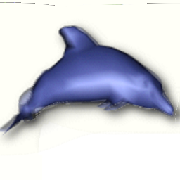
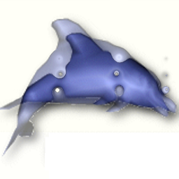
If alpha is large, e.g. alpha > 0.01, function values at most points (other than control points) is reduced to near zero, causing artifacts (Fig. 10).
alpha = 0.05 alpha = 0
Fig. 10 The comparison of different alpha.
