2. More Issues
Besides the basic algorithm, I implement bundle adjustment, up-vector selection, and two-band blending. I also consider the acceleration.
|
|||
2.1 Bundle Adjustment
The errors are accumulated during the process of stitching. I find that the drift error is usually inevitable in the panorama mosaic (the red boxes in Fig. 3) because the coordinate is distorted by sphere transformation. For example, two features lie on one a horizontal line become lying on a curve after transformation. A linear drift compensation y' = y + ax may be used to address this issue. However, I implement a more complicated bundle adjustment algorithm.
The bundle adjustment minimizes the global error of feature matching, i.e. the sum of
 (5) (5)for all matched inliers (pij, pik) where is pij from image j and pik is from image k.
To solving this problem, Levenberg-Marquardt nonlinear least squares algorithm is used, which multiplies the diagonal of the normal equations by a factor (1+λ), with λ being increase/decreased according to the success of the previous iteration.
The rotation matrix is written as
 (6) (6)and thus the update of the transformation matrix is
 , where , where  Then in each iteration of L-M algorithm, the update is solved from (5) = 0 (note that this equation should be applied to different i, j and k), i.e.
 (7) (7)Several typical results without and with bundle adjustment are presented in Fig. 3.
 Without bundle adjustment High-resolution image
 With bundle adjustment High-resolution image
 Without bundle adjustment High-resolution image
 With bundle adjustment High-resolution image
 Without bundle adjustment High-resolution image
 With bundle adjustment High-resolution image
Fig. 3 Comparison of results without and with bundle adjustment (please see the region in the red box).
|
|||
2.2 Up-vector Selection
A simple way of doing the global orientation specification is to rotate the panorama so that the first image is at the equator. However, such a choice is not always the best.
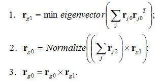
Another intuition is from the people's preference that the final stitched image is better to be "upright" than twisted or tilted. So the horizontal edge of the image usually stays parallel to the ground plane. Mathematically, the image x-axis (1,0,0) is perpendicular to transformed global y-axis, i.e.
 (8) (8)where RjRg is corrected transformation matrix for image j and Rg is the global orientation we want to solve. It is converted to a least square problem
 (9) (9)where rg1 is the second column of Rg, and rj0 is the first row of Rj. The three steps for computing Rg are:
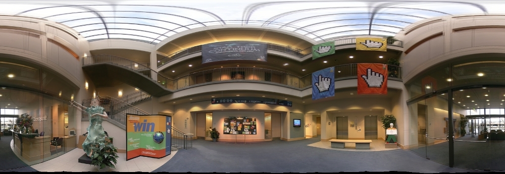
 A comparison of results without and with up-vector selection is shown in Fig. 4.
 Without up-vector selection High-resolution image
 With up-vector selection High-resolution image
Fig. 4 Comparison of results without and with up-vector selection.
|
|||
2.3 Two-band Blending
The simple alpha blending I use in the basic algorithm may cause blur (see the first row of Fig. 5) in many output panoramas. To overcome the problem, I use the two-band blending method in [3] to blend the image. The image is separated into the high-band and low-band image. The high-band image is blended by choosing the pixel value with the maximum weight. Low-band is blended by the weighted sum. The results becomes sharper with two-band approach (Fig. 5). However, two-band approach may cause problems such as discontinuities of edges. It can be further improved with multiband blending.
  Without up-vector selection High-resolution image Zooming
  With up-vector selection High-resolution image Zooming
Fig. 5 Comparison of single-band and two-band blending.
|
|||
2.4 Acceleration
A time-consuming process is the pairwise alignment and the intial nearest neighbor search costs the most time if use direct implementation. I use ANN library to perform nearest neighbor search and compare the time of both approaches on a 3.0GHz CPU, 1G memory PC. Typically, for 2000-4000 feature points in an image, the nearest neighbor search for a pair of images needs 12-15 seconds. While the time is only 1-2 seconds using ANN. The other part of the pairwise alignment needs less than 1 second.
Another acceleration is to use a sparse matrix library to solve the sparse linear system in L-M algorithm for bundle adjustment.
WIth both acceleration and careful consideration in programming, the running time of the program is acceptable for trial and test.
|
|||