1.1 The Algorithm
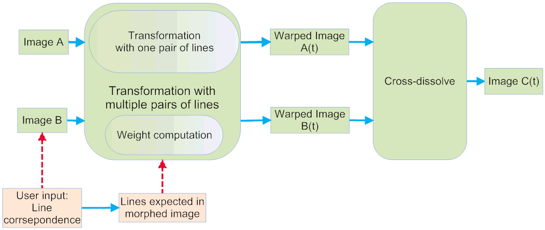
The paper can be found at http://www.hammerhead.com/thad/morph.html. Following this paper, my implementation can be summarized as the flowchart in Fig. 2. I only give the key steps in this report, while other details can be found in the paper.
Fig. 2 Illustration of Beier-Neely Algorithm
A. The interpolation of control lines
To warp the two images and align them well, each pair of control lines inputted by the user should be interpolated to obtain the corresponding line in the morphed image. I implement two different ways of the interpolation: two-endpoint interpolation and center-orientation interpolation. The limitation of the first way is that a rotating line would shrink in the middle of the metamorphosis (Fig. 3).
Two-endpoint interpolation
Center-orientation interpolation
Left Image Morphed Image Right Image
Fig. 3 The comparison of endpoint-based interpolation and center orientation interpolation of control lines.
The red lines are the control lines.
B. Coordinate Transformation with One Pair of Lines
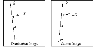
After the control line interpolation, we obtain the corresopondence between the destination image (the morphed image C(t)) and the source image (the left image A or the right image B). Given one pair of lines (PQ and P'Q') and a point X in the destination image (Fig. 4), you can find the coordinates of the corresponding point X’' in the source image using the following process:
Fig. 4 Coordinate Transformation with One Pair of Lines
For each pixel X in the destination image
find the corresponding u, v
find the X' in the source image for that u, v
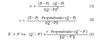
The forms of u, v and X' is given as follows:
where Perpendicular() returns the vector perpendicular to, and the same length as, the input vector.
C. Coordinate Transformation with Multiple Pairs of Lines
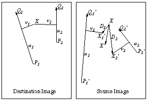
Multiple pairs of lines specify more complex transformations. X' in the source image is computed as the weighted sum of multiple Xi' for different single line transformation.
For PQ in the destination image and Pi'Qi' in the source image (Fig. 5), the corresponding Xi' is computed as in Section 1.1-B.
Fig. 5 Coordinate Transformation with Multiple Pairs of Lines
Then the weight for Xi' is
where length = ||PQ||, dist is the distance from the pixel to the line (note that the computation of dist should be careful and the detail will be given in Section 1.2), and a, b, and p are parameters that can be used to change the relative effect of the lines.
Finally all the weights should be normalized as wi = wi / weightsum, where weightsum is the sum of all the weights wi.
The transformed coordinate
(5)
D. Image Warping
There are two ways to warp an image.
The first, called forward mapping, scans through the source image pixel by pixel, and copies them to the appropriate place in the destination image.
The second, reverse mapping, goes through the destination image pixel by pixel, and samples the correct pixel from the source image. The most important feature of inverse mapping is that every pixel in the destination image gets set to something appropriate. In the forward mapping case, some pixels in the destination might not get painted, and would have to be interpolated. In the implementation, we calculate the image deformation as a reverse mapping.
1.2 Discussion
A. The computation of dist
There is an important footnote on dist: "note that these lines are directed line segments. The distance from a line to a point is abs(v) if 0 < u < 1, the distance from P to the point if u < 0, and the distance from Q to the point if u > 1." When X is close to the line PQ but not close to the line segment PQ, the weight of the line segment PQ should be small and cannot be determined by the distance from the line PQ to X. Ignoring this will cause severe artifacts (Fig. 6).
Fig. 6 The comparison of using the distance from the line PQ (left) and the line segment PQ (Right) to a point X
B. The parameters a, b and p in the weight of a line segment
The choices of the parameters reported in [1] are: a > 0, 0.5 < b < 2 and 0 < p < 1.
The performance of the algorithm is robust in a range for those parameters.
My experiences are: 0< a <1, 1 < b < 10 (depends on the images), 0.5 < p < 1.
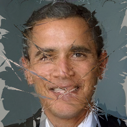
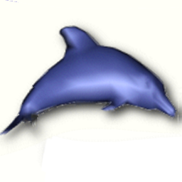
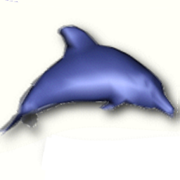
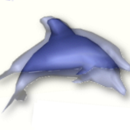
The effects of different choices of parameters are shown in Fig. 7.
The bigger a is, the less the effect of dist is. Thus, there are misalignments in the morphed image when a = 10.
The smaller b is, the less the effect of dist is. Thus, there are misalignments in the morphed image when b = 0.1 and b = 1.
The bigger b is, the more the effect of dist is. In this case, there are other artifacts as one or two line segments may dominate the transformation. Thus the transformation may be incorrect as the user input may be noisy. You can see the result of b = 10.
If p is too small or too large, there may be some short or long line segments affect the transformation.
Fig. 7 The effects of different parameters




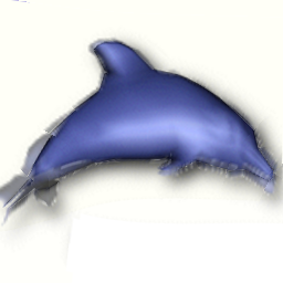 b = 1
b = 1
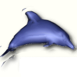
 p = 0.1
 p = 0.5
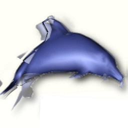 p = 3
p = 3